Random Variables
We talked before about probability using simple sample spaces, but in reality, we will map situations to probabilistic models that cater to all possible results. The variables to which we are going to construct probabilistic models are called random variables.
A random variable is a real-valued variable whose value is determined by an underlying random experiment. We usually show random variables by capital letters such as \(X\), \(Y\), and \(Z\). Since a random variable is a function, we can talk about its range. The range of a random variable \(X\) is the set of possible values for \(X\).
Discrete Random Variables
\(X\) is a discrete random variable, if its range is countable.
Example: Imagine that we extracted 2 balls without repositioning from an urn that initially contained 2 blue balls and 3 violet balls. Let’s define \(X\) as the number of violet balls obtained after both extractions. The following chart shows us the possible outcomes for \(X\).
| Result | Probability | X |
|---|---|---|
| BB | 1/10 | 0 |
| BV | 3/10 | 1 |
| VB | 3/10 | 1 |
| VV | 3/10 | 2 |
Each result of the experiment is associated with a value of \(X\). Each of these results has a probability associated, which allow us to write the function (x, p(x)) that is a model for the distribution of \(X\). The function (x, p(x)) is called probability function of \(X\).
In the table below, we have the probability distribution of \(X\) for the example we just saw.
| x | p(x) | |
|---|---|---|
| 0 | 1/10 | |
| 1 | 6/10 | |
| 2 | 3/10 |
Special distributions
Some random variables adapt very well to a series of practical problems, and they have been given unique names.
Discrete Uniform distribution
Each value has the same probability of happening. X is uniformly distributed if and only if
\[\mathbb{P}(X = x_i) = \frac{1}{n} \forall i=1,…,n\]
Bernoulli
It can only take two possible values, usually 0 and 1. This random variable models random experiments that have two possible outcomes, sometimes referred to as “success” and “failure”.
A random variable \(X\) is a Bernoulli random variable with parameter \(p\), where \(p\) is the probability of success, shown as \(X∼Bernoulli(p)\), if
\[ \mathbb{P}(X = x_i)= \begin{cases} p, & \text{ for } x = 1\\ 1 - p, & \text{ for x = 0}\\ 0, & \text{ otherwise} \end{cases} \]
Example: A die is tossed, and we are interested at die showing 5, so it either it shows a 5 or not.
Binomial distribution
Assume that we repeat a Bernoulli experiment n times, also, assume that the repetitions are independent, i.e., the result of an experiment won’t impact another one. A random variable \(X\) is said to be a binomial random variable with parameters \(n\) and \(p\), shown as \(X∼Binomial(n,p)\), if
\[\mathbb{P}(X = k) = \binom{n}{k}p^k(1-p)^{n-k}, k=0,1,...,n\]
Example: A coin is thrown 3 times. What is the probability of 2 heads?
Geometric distribution
Repeating independent Bernoulli trials until observing the first success. A random variable \(X\) is said to be a geometric random variable with parameter \(p\), shown as \(X∼Geometric(p)\) if
\[\mathbb{P}(X = k) = p(1-p)^{k-1}, k=1,2, ...\]
Poisson distribution
Used in scenarios where we are counting the occurrences of certain events in an interval of time or space. A random variable \(X\) is said to be a Poisson random variable with parameter \(\lambda\), shown as \(X∼Poisson(\lambda)\), if
\[\mathbb{P}(X = k) = \frac{e^{-\lambda}\lambda^k}{k!}, k=0,1,...\]
Example: A phone number receives, on average, 5 calls per minute. What is the probability of not receiving a call in one minute?
Continuous Random Variables
A continuous random variable is one which takes an infinite number of possible values; It is defined over an interval of values, and is represented by the area under a curve. The probability of observing any single value is equal to 0, since the number of values which may be assumed by the random variable is infinite.
Special distributions
We also have special distributions for continuous random variables.
Uniform distribution
A random variable \(X\) is said to have a Uniform distribution over the interval \([a,b]\), shown as \(X∼\mathcal{U}(a,b)\), if:
\[ f(x;a, b)= \begin{cases} \frac{1}{b-a}, & \text{if } a \leq x \leq b\\ 0, & \text{ otherwise} \end{cases} \]
Exponential distribution
A random variable \(X\) is said to have an exponential distribution with parameter \(\lambda > 0\), shown as \(X∼Exp(\lambda)\), if
\[ f(x; \lambda)= \begin{cases} \lambda e^{-\lambda x}, & \text{ for } x > 0\\ 0, & \text{ otherwise} \end{cases} \]
Normal (Gaussian) distribution
The normal distribution is by far the most important probability distribution. One of the main reasons for that is the Central Limit Theorem (CLT) that we will discuss in another moment.
A random variable \(X\) is said to have a normal distribution with parameter \(\mu \in \mathbb{R}\) and \(\sigma^2 > 0\) if
\[f(x; \mu, \sigma^2) = \frac{1}{\sigma\sqrt{2\pi}}e^{-\frac{(x-\mu)^2}{2\sigma^2}}, -\infty < x < \infty\]
Below we can see the representation of a normal distribution with mean \(\mu\) and standard deviation \(\sigma\)
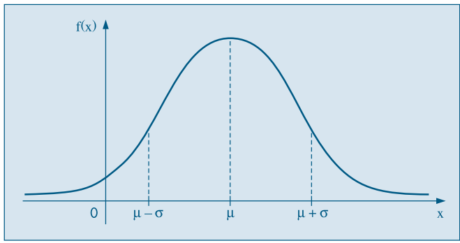
When \(\mu = 0\) and \(\sigma = 1\) we say that we have a standard normal distribution ans we represent as \(Z∼\mathcal{N}(0,1)\) and the probability function is reduced to
\[f(z) = \frac{1}{\sqrt{2\pi}}e^{-\frac{z^2}{2}}, -\infty < z < \infty\]
If \(X∼\mathcal{N}(\mu, \sigma^2)\), then the variable defined as \(Z = \frac{X - \mu}{\sigma}\) has mean 0 and variance 1
Emmanuelle R. Nunes
Senior Data Scientist
My interests include statistics, machine learning, health and social statistics.